
Transforming Graphs into 3D Environments for AI Agents
A Neural Simulation Approach

Introduction
Graphs are powerful data structures used to model relationships between entities. From social networks to molecular structures, graphs enable us to represent complex systems in a structured way. But what if we could transform these abstract graphs into tangible 3-dimensional environments where AI agents can navigate, learn, and adapt?
In this article, we'll explore how to convert graphs into dynamic 3D environments suitable for reinforcement learning. We'll walk through a Python implementation that leverages hyperbolic space to simulate graph dynamics, allowing AI agents to interact with the environment in a meaningful way.
Table of Contents
Background
Graphs in Machine Learning
Graphs consist of nodes (vertices) and edges, representing entities and their relationships. In machine learning, graphs are used in various domains:
Social Network Analysis: Understanding relationships between individuals.
Knowledge Graphs: Representing information in a structured form.
Graph Neural Networks (GNNs): Learning over graph-structured data.
Hyperbolic Space
Hyperbolic space is a non-Euclidean geometry with constant negative curvature. It's particularly useful for embedding hierarchical data structures like trees and graphs. The Poincaré ball model is a popular representation of hyperbolic space.
Reinforcement Learning in 3D Environments
Reinforcement Learning (RL) involves agents learning to make decisions by interacting with an environment. By converting graphs into 3D spaces, we enable RL agents to:
Navigate Complex Structures: Move through the environment based on the graph's topology.
Learn from Interactions: Update policies based on rewards from the environment.
Setting Up the Neural Graph Simulator
We'll begin by setting up a neural graph simulator that embeds graph nodes into hyperbolic space. This allows us to represent the graph in a continuous 3D environment.
Importing Libraries
import torch
import torch.nn as nn
import torch.optim as optim
import networkx as nx
import numpy as np
import geoopt
from geoopt import ManifoldParameter
from geoopt.manifolds import PoincareBall
import matplotlib.pyplot as plt
import random
from tqdm import tqdm
from torch.nn import Parameter
from geoopt.optim import RiemannianAdam
Setting the Random Seed
For reproducibility, we set a random seed:
torch.manual_seed(42)
np.random.seed(42)
random.seed(42)
Defining the Neural Graph Simulator Class
class NeuralGraphSimulator:
    def __init__(self, num_nodes):
        self.manifold = PoincareBall(c=1.0)
        self.graph = nx.Graph()
        self.num_nodes = num_nodes

        # Initialize nodes with random hyperbolic coordinates
        for i in range(num_nodes):
            point = ManifoldParameter(
                self.manifold.random(2),
                manifold=self.manifold
            )
            value = Parameter(torch.rand(1))
            self.graph.add_node(i, coords=point, value=value)

        # Initialize edges with random weights
        for i in range(num_nodes):
            for j in range(i + 1, num_nodes):
                if np.random.rand() < 0.3:
                    weight = Parameter(torch.rand(1))
                    self.graph.add_edge(i, j, weight=weight)
Key Components
ManifoldParameter: Used to represent points in hyperbolic space.
Node Initialization: Each node is assigned random coordinates and a value.
Edge Initialization: Edges are randomly created with weights.
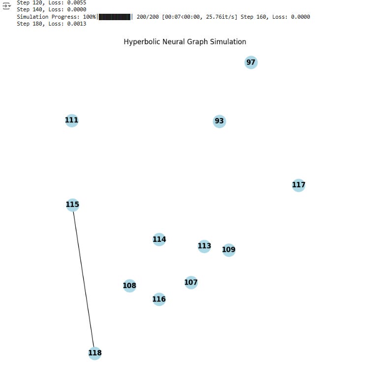
Visualizing the Graph
We add a method to visualize the graph:
def visualize(self):
    coords = [self.graph.nodes[n]['coords'].detach().numpy() for n in self.graph.nodes]
    x = [coord[0] for coord in coords]
    y = [coord[1] for coord in coords]

    pos = dict(zip(self.graph.nodes, zip(x, y)))

    plt.figure(figsize=(8, 8))
    nx.draw(self.graph, pos, with_labels=True, node_color='lightblue', font_weight='bold', node_size=500)
    plt.title("Hyperbolic Neural Graph Simulation")
    plt.axis('equal')
    plt.show()
Designing the Neural Network
We create a simple neural network that will be used by the AI agent to interact with the graph.
class SimpleNet(nn.Module):
    def __init__(self, input_size, output_size):
        super(SimpleNet, self).__init__()
        self.fc1 = nn.Linear(input_size, 64)
        self.relu = nn.ReLU()
        self.fc2 = nn.Linear(64, output_size)

    def forward(self, x):
        x = self.relu(self.fc1(x))
        x = self.fc2(x)
        return x
Input Layer: Takes the average value of neighboring nodes.
Hidden Layer: Consists of 64 neurons with ReLU activation.
Output Layer: Produces an updated value for the node.
Simulation Loop and Dynamics
The simulation involves the AI agent navigating and updating the graph over multiple steps.
Simulation Step Function
def simulation_step(sim, model, optimizer, manifold_optimizer):
    # AI navigates through the graph
    for node in list(sim.graph.nodes):
        neighbors = list(sim.graph.neighbors(node))
        neighbor_values = [sim.graph.nodes[n]['value'] for n in neighbors]

        if neighbor_values:
            input_tensor = torch.stack(neighbor_values).mean(dim=0)
            output = model(input_tensor)

            # Update node value
            sim.graph.nodes[node]['value'].data.copy_(output.data)

            # Adjust edge weights and node coordinates
            for neighbor in neighbors:
                delta = (output - sim.graph.nodes[neighbor]['value']).abs()
                sim.graph[node][neighbor]['weight'].data.add_(delta.data)

                with torch.no_grad():
                    coord = sim.graph.nodes[node]['coords']
                    neighbor_coord = sim.graph.nodes[neighbor]['coords']
                    direction = sim.manifold.logmap(coord, neighbor_coord)
                    updated_coord = sim.manifold.expmap(coord, 0.01 * direction)
                    coord.data.copy_(updated_coord.data)

    # Loss function: minimize differences between connected nodes
    loss = torch.tensor(0.0, requires_grad=True)
    for edge in sim.graph.edges:
        n1, n2 = edge
        loss = loss + (sim.graph.nodes[n1]['value'] - sim.graph.nodes[n2]['value']).pow(2).sum()

    optimizer.zero_grad()
    manifold_optimizer.zero_grad()
    loss.backward()
    optimizer.step()
    manifold_optimizer.step()

    # Dynamic restructuring of the graph
    sim.dynamic_restructuring()
    update_optimizers(optimizer, manifold_optimizer, sim, model)

    return loss.item()
Dynamic Restructuring
Nodes with low values are removed, and new nodes are added with a certain probability.
def dynamic_restructuring(self):
    nodes_to_remove = [n for n, attr in self.graph.nodes(data=True) if attr['value'].item() < 0.05]
    if len(nodes_to_remove) >= len(self.graph.nodes):
        if len(self.graph.nodes) > 0:
            nodes_to_remove = nodes_to_remove[:-1]
        else:
            nodes_to_remove = []
    for node in nodes_to_remove:
        self.remove_node(node)
    if np.random.rand() < 0.5:
        self.add_node()
Updating Optimizers
When the graph changes, we need to update the optimizer parameters.
def update_optimizers(optimizer, manifold_optimizer, sim, model):
    euclidean_params = list(model.parameters())
    manifold_params = []

    for node in sim.graph.nodes:
        euclidean_params.append(sim.graph.nodes[node]['value'])
        manifold_params.append(sim.graph.nodes[node]['coords'])

    for edge in sim.graph.edges:
        euclidean_params.append(sim.graph[edge[0]][edge[1]]['weight'])

    optimizer.param_groups[0]['params'] = euclidean_params
    manifold_optimizer.param_groups[0]['params'] = manifold_params
Visualizing the Simulation
Initializing the Simulation
sim = NeuralGraphSimulator(num_nodes=50)
model = SimpleNet(input_size=1, output_size=1)
Collecting Parameters
euclidean_params = list(model.parameters())
manifold_params = []

for node in sim.graph.nodes:
    euclidean_params.append(sim.graph.nodes[node]['value'])
    manifold_params.append(sim.graph.nodes[node]['coords'])

for edge in sim.graph.edges:
    euclidean_params.append(sim.graph[edge[0]][edge[1]]['weight'])
Setting Up Optimizers
optimizer = optim.Adam(euclidean_params, lr=0.01)
manifold_optimizer = RiemannianAdam(manifold_params, lr=0.01)
Running the Simulation
losses = []
num_steps = 200
for step in tqdm(range(num_steps), desc="Simulation Progress"):
    if len(sim.graph.nodes) == 0:
        print("Graph is empty. Adding a new node.")
        sim.add_node()
        update_optimizers(optimizer, manifold_optimizer, sim, model)
    loss_value = simulation_step(sim, model, optimizer, manifold_optimizer)
    losses.append(loss_value)
    if step % 20 == 0:
        print(f"Step {step}, Loss: {loss_value:.4f}")
Visualizing the Final Graph
if len(sim.graph.nodes) > 0:
    sim.visualize()
else:
    print("Graph is empty at the end of the simulation.")
Plotting the Loss Curve
plt.figure(figsize=(6, 4))
plt.plot(losses)
plt.title("Loss Over Time")
plt.xlabel("Steps")
plt.ylabel("Loss")
plt.show()
Loss decreases over time, indicating that node values are becoming more similar among connected nodes.
Conclusion
Transforming graphs into 3D environments opens up new possibilities for AI agents in reinforcement learning. By embedding nodes in hyperbolic space and simulating dynamics through neural networks, we create a rich environment for agents to explore and learn.
This approach allows for:
Dynamic Environments: The graph restructures itself based on node values.
Rich Interactions: Agents can interact with both the topology and the attributes of the graph.
Scalability: The framework can be scaled to larger graphs and more complex neural networks.
Future work could involve integrating more sophisticated reinforcement learning algorithms and extending the simulation to higher-dimensional hyperbolic spaces.
References
Geoopt Library: https://github.com/geoopt/geoopt
NetworkX Documentation: https://networkx.org/documentation/stable/
Hyperbolic Neural Networks: Nickel, M., & Kiela, D. (2017). Poincaré embeddings for learning hierarchical representations. Advances in Neural Information Processing Systems, 30.